THNN是一个用C语言实现的神经网络模块的库,提供的功能非常底层。它实现了许多基础的神经网络模块,包括线性层,卷积层,Sigmoid等各种激活层,一些基本的loss函数,这些API都声明在THNN/generic/THNN.h中。每个模块都实现了前向传导(forward)和后向传导(backward)的功能。THCUNN则是对应模块的CUDA实现。
目录
THNN & THCUNN
我们通过几个例子具体看一下几种模块是怎么实现的。
Tanh
首先从最简单的激活层开始看,以 \(\tanh\) 为代表,代码在THNN/generic/Tanh.c。这个模块只有两个函数,分别是THNN_(Tanh_updateOutput)()和THNN_(Tanh_updateGradInput)(),其中前者实现了前向传播,后者实现了反向传播。注意到函数的命名方式,依旧是使用宏实现范式,THNN_是宏定义,Tanh_是具体模块名,updateOutput表示前向传播,updateGradInput表示反向传播,与之前不同的是,这里只需生成浮点类型(float和double)的实现即可。
前向传播的实现很简单,直接调用之前实现的tanh函数就行了:
1 | void THNN_(Tanh_updateOutput)( |
它有三个参数,分别是THNN状态(暂不知有何用),本层的输入(input)和本层的输出(output),输出存储在output参数中。
反向传播的实现为:
1 | void THNN_(Tanh_updateGradInput)( |
反向传播接收5个参数,分别是THNN状态,从后面传回来的梯度(gradOutput),本层往回传的梯度(gradInput),本层前向传播的输出(output),这个函数计算的是本层的梯度,然后存储在gradInput中。
\(\tanh\) 的导数为: \[
f(z) = \tanh(z)\\
f'(z) = 1 - (f(z))^2
\] 其中,\(f(z)\) 就是前向传播时本层的输出,也就是output参数(循环里的z),根据链式法则,再乘以后面层传回来的梯度(gradOutput)就是本层应该往回传的梯度了(相对于本层输入的梯度),所以循环里的代码为:
1 | *gradInput_data = *gradOutput_data * (1. - z*z); |
注:_data后缀表示数据指针,具体可以看Apply宏的实现。
2D Convolution
最普通的2D卷积,CPU实现在THNN/generic/SpatialConvolutionMM.c,CUDA实现在THCUNN/generic/SpatialConvolutionMM.cu,大体的算法是把输入展开成一个特殊的矩阵,然后把卷积转化为矩阵相乘(MM = Matrix Multiplication)。模块里主要包含三个函数,前向传播(THNN_(SpatialConvolutionMM_updateOutput)()),反向传播(THNN_(SpatialConvolutionMM_updateGradInput)()),和更新层内参数(THNN_(SpatialConvolutionMM_accGradParameters)())。
前向传播
PyTorch实现卷积的做法是用im2col算法把输入展开成一个大矩阵,然后用kernel乘以这个大矩阵,就得了卷积的结果。这里不具体介绍im2col算法是怎么做的,但会解释为什么可以这么做。
首先定义符号,为了和代码中的符号一致,首先来看一下updateOutput的声明:
1 | void THNN_(SpatialConvolutionMM_updateOutput)( |
其中,
input是输入的4D Tensor,大小为 \(\text{batch}\times\text{nInputPlane}\times\text{inputHeight}\times\text{inputWidth}\),batch维也可以没有,就变为3D Tensor;output是输出的4D或3D Tensor,大小为 \(\text{batch}\times\text{nOutputPlane}\times\text{outputHeight}\times\text{outputWidth}\),其中,
\[ \text{outputHeight}=\frac{\text{inputHeight}+2\ast\text{padH}-\text{kH}}{\text{dH}}+1\\ \text{outputWidth}=\frac{\text{inputWidth}+2\ast\text{padW}-\text{kW}}{\text{dW}}+1 \]
weight是权重,也就是卷积核,大小为 \(\text{nOutputPlane}\times\text{nInputPlane}\times\text{kH}\times\text{kW}\);bias是偏置,大小为 \(\text{nOutputPlane}\times1\times1\times1\);columns用于存储im2col的结果;ones是一个值全为1的矩阵,大小为 \(\text{outputHeight}\times\text{outputWidth}\),用于计算偏置;kW和kH是卷积核(kernel)的宽和高;dW和dH是步长(stride);padW和padH是补零的宽和高。
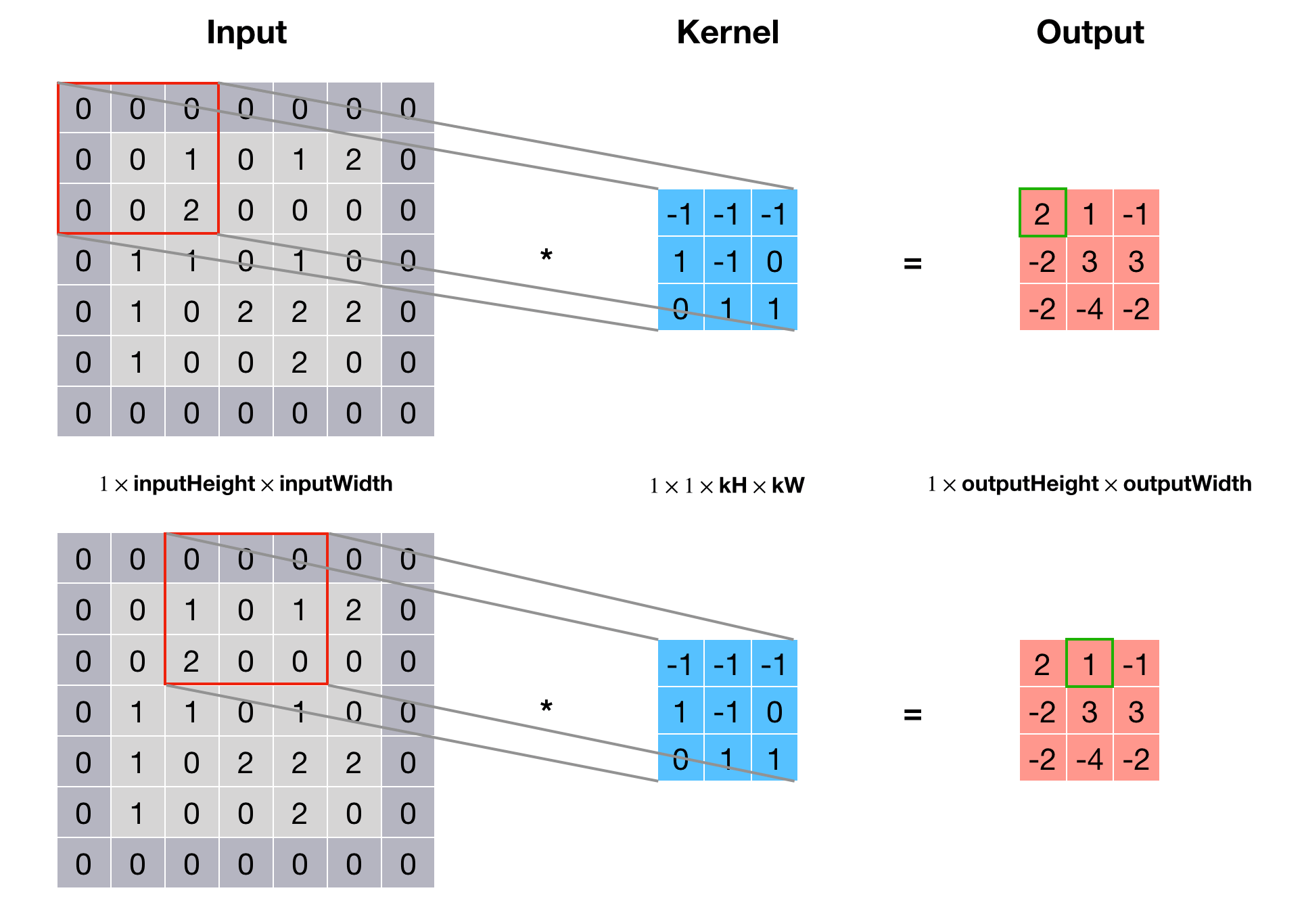
定义好了符号之后来看一下卷积是怎么转化为一个矩阵乘法的。首先来看卷积是怎么做的,下图是一个简单的例子,其中输入和输出深度 \(\text{nInputPlane}=\text{nOutputPlane}=1\),卷积核大小 \(\text{kH}=\text{kW}=3\),输入大小 \(\text{inputHeight}=\text{inputWidth}=7\),步长 \(\text{dW}=\text{dH}=2\),补零 \(\text{padW}=\text{padH}=1\),可以算出 \(\text{outputHeight}=\text{outputWidth}=3\)。
要想把卷积变成一次矩阵乘法运算,就需要把输入中每个卷积窗口变为单独一列,这也就是im2col做的事情,见下图:
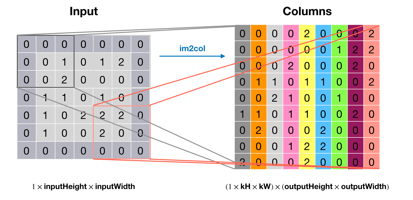
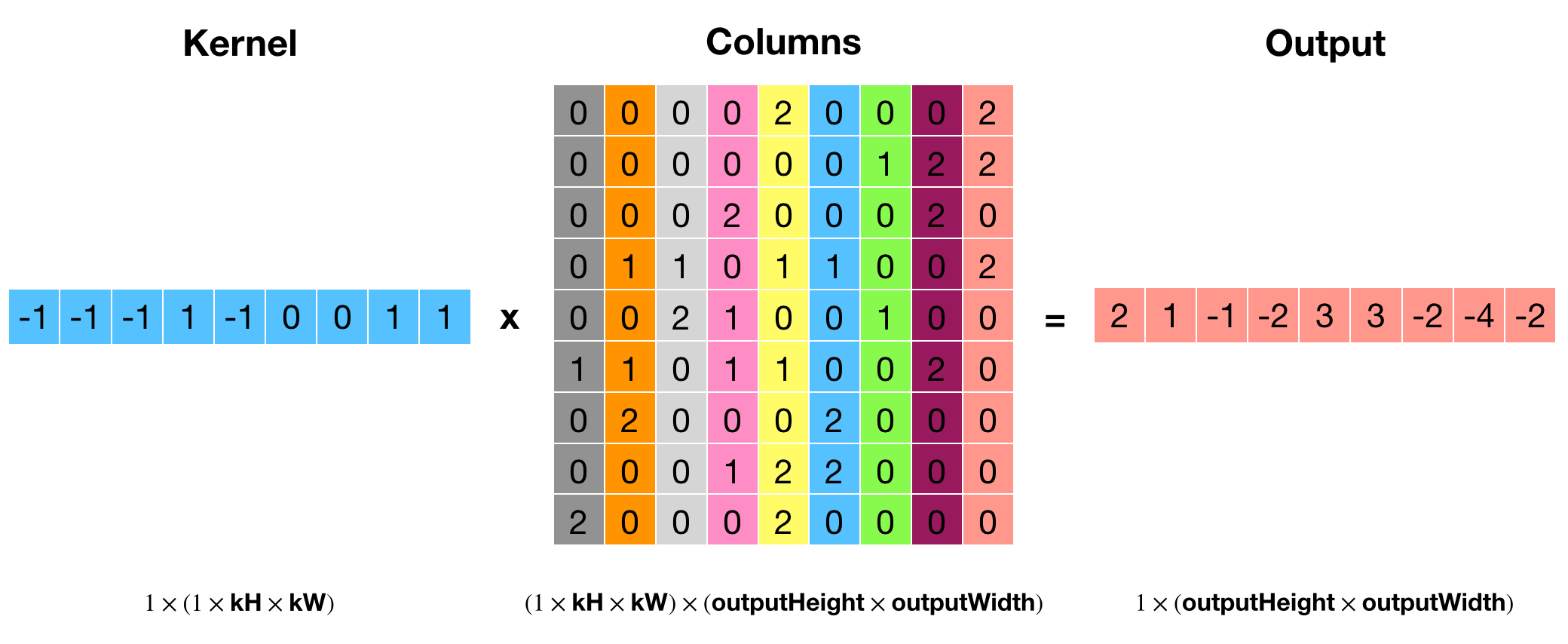
上图中右边矩阵的每一列都是原输入矩阵的一个卷积窗口,转换后的矩阵大小为 \[ (\text{nInputPlane}\times\text{kH}\times\text{kW})\times(\text{outputHeight}\times\text{outputWidth}) \] 得到上述矩阵之后,只需把kernel的大小也resize成 \[ (\text{nOutputPlane})\times(\text{nInputPlane}\times\text{kH}\times\text{kW}) \] 就可以直接用kernel乘以该矩阵得到卷积结果了,见下图。
代码(CUDA版)
1 | void THNN_(SpatialConvolutionMM_updateOutput)(/* 参数列表前面有 */) { |
反向传播
首先来看一下卷积层反向传播的公式,设第 \(l\) 层的输入为 \(a^{l-1}\),卷积核为 \(W\),偏置为 \(b\),输出为 \(z^l = a^{l-1}*W+b\),相对于输出的误差梯度为 \(\delta^l = \frac{\partial \text{Loss}}{\partial z^l}\),则相对于输入的梯度为: \[ \delta^{l-1}=\delta^l*\text{rot180}(W^l) \] 相对于权重和偏置的梯度为: \[ \frac{\partial\text{Loss}}{\partial W^l}=\frac{\partial\text{Loss}}{\partial z^l}\frac{\partial z^l}{\partial W^l}=a^{l-1}*\delta^l\\ \frac{\partial\text{Loss}}{\partial b^l}=\sum_{u,v}(\delta^l)_{u,v} \] 注:\(*\) 为卷积的意思,\(\text{rot180}(x)\) 为把矩阵 \(x\) 旋转180度的意思。公式推导可以看这篇博客。
从公式可以看出反向传播分为两个部分:计算对输入的梯度和计算对参数的梯度,这两部分也分别对应了模块里的两个函数,我们一个一个分析。
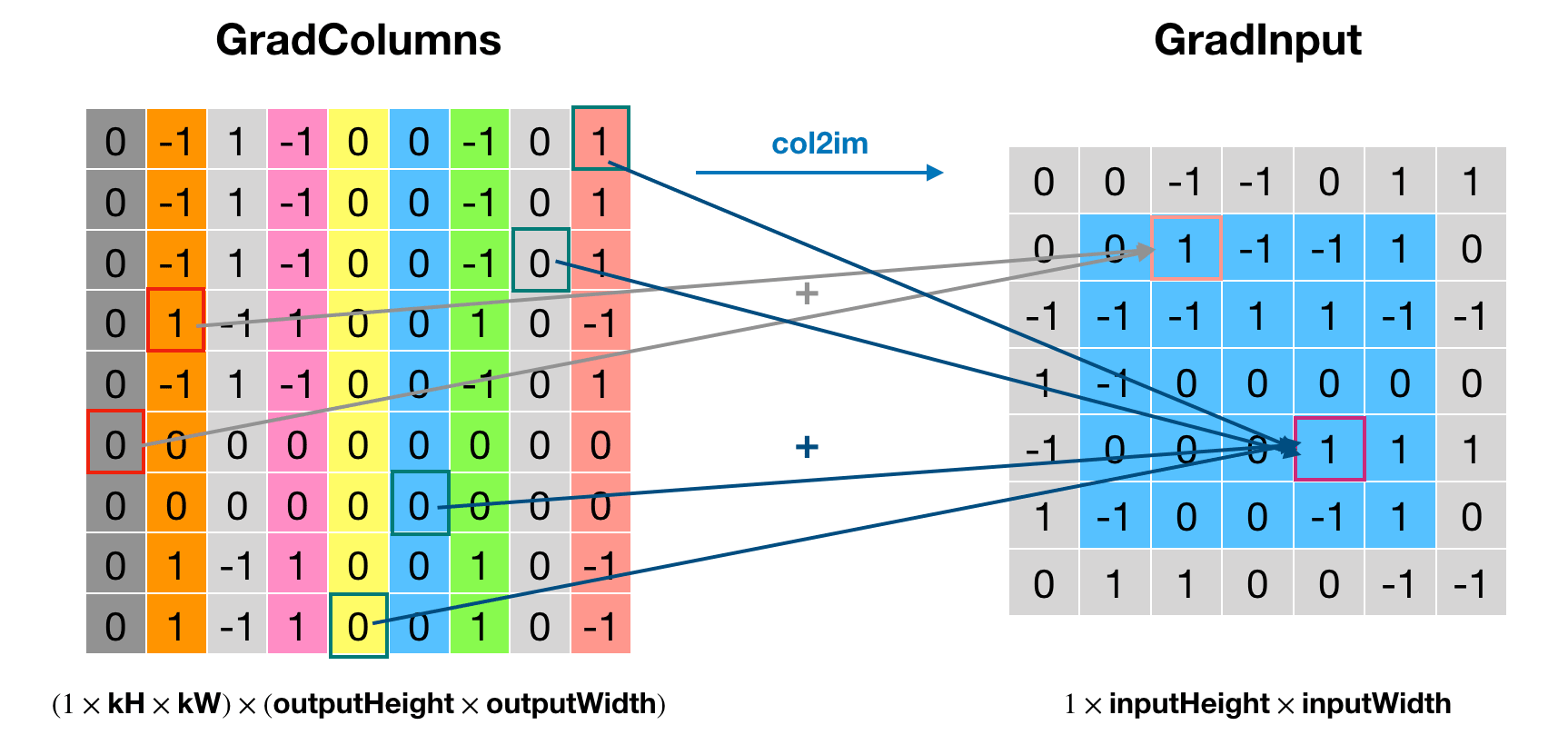
THNN_(SpatialConvolutionMM_updateGradInput)
这部分是计算对输入的梯度,虽然公式摆在了那里,但Torch的代码实现并不是直接翻译公式,我也一直没能把这部分的实现和公式对上,不过倒是可以通过图示的方式来理解,有点像前向传播的逆过程,把卷积后的梯度分配回卷积前。
在画图之前还是先定义一些符号:
1 | void THNN_(SpatialConvolutionMM_updateGradInput)( |
其中(与前向传播相同的参数就不重复介绍了),
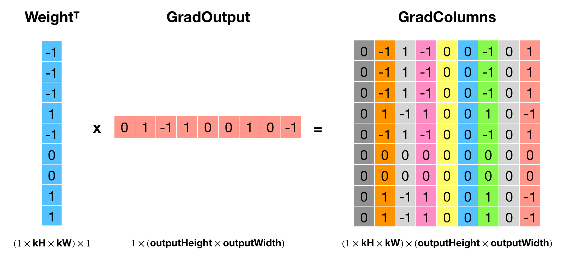
gradOutput是相对于输出的梯度,即 \(\delta^l\),大小与前向传播的输出output相同;gradInput是相对于输入的梯度,即 \(\delta^{l-1}\),是这个函数需要计算的对象,大小与输入input相同;gradColumns是个列矩阵,用于存储临时的梯度,大小为 \((\text{nInputPlane}\times\text{kH}\times\text{kW})\times(\text{outputHeight}\times\text{outputWidth})\);
代码的实现逻辑是用权重的转置乘以输出梯度,得到gradColumns,然后通过col2im还原到输入的大小,即得到了相对输入的梯度 gradInput。这个操作看起来就是前向传播的逆操作,但是搞不懂为什么这样就实现了 \(\delta^l*\text{rot180}(W^l)\),如果有大佬知道希望评论区指点一下。使用前面例子的设定,这波操作的示意图如下所示:
核心部分代码(其余部分与前向传播类似)
1 | /* 循环取每个批次: */ |
THNN_(SpatialConvolutionMM_accGradParameters)
接下来看计算参数梯度的部分,这部分相对好理解,因为代码和公式一样,还是先看函数声明:
1 | void THNN_(SpatialConvolutionMM_accGradParameters)( |
其中,
gradWeight是权重的梯度,是这个函数需要计算的对象,大小和权重相同;gradBias是偏置的梯度,也是函数需要计算的对象,大小与偏置相同(就是一个Vector)columns是用来存储 im2col 的结果,因为要计算卷积,所以要把输入展开scale_是学习速率(learning rate)
已知权重梯度的计算公式为 \(\frac{\partial\text{Loss}}{\partial W^l}=a^{l-1}*\delta^l\),这个卷积的计算方式和前向传播相同:首先把输入(\(a^{l-1}\))通过im2col展开为列矩阵,存储到columns里,然后用 gradOutput 乘以 columns 计算卷积。而偏置梯度的计算就是把 gradOutput 累加成一个长度为 \(\text{nOutputPlane}\) 的 Tensor 即可。
核心代码
1 | void THNN_(SpatialConvolutionMM_accGradParameters)(/* 略 */) { |
ATen
看了THNN.h的读者可能会发现,THNN和THCUNN只定义了少量的神经网络相关的函数,其实大部分都定义在ATen中,这个ATen是指pytorch/aten/src/ATen文件夹(下同)。说到底,TH系列库都是torch lua时代留下的产物,是用C语言实现的,后来PyTorch开发者觉得cpp大法好,就用C++写了ATen,把TH里的接口都封装了,同时新的API直接在ATen里实现。
这个ATen有点意思,它大概干了这么几件事情:
- 在
ATen/core/Tensor.h定义了at::Tensor类型,这个是C++前端以及更上层的API都在用的Tensor类型,它的成员内有一个TensorImpl impl_,提供底层实现; - 实现和封装了有关Tensor的所有操作,并根据数据类型和设备进行自动派发;
- 使用Python脚本生成ATen API。
其中从TH(包括THC、THNN等)里封装的函数叫做 legacy函数,而在ATen直接实现的函数叫 native函数。native函数的实现全在ATen/native文件夹中,实现了THNN里没有的神经网络和Tensor操作,比如RNN什么的,API列表在ATen/native/native_functions.yaml里,感兴趣的童鞋可以自己阅读。
了解了神经网络每一层的前向传播和反向传播的实现之后,下一步就是控制执行顺序了,也就是自动微分(Autograd),下一章将介绍PyTorch自动微分的实现。
つづく
| 上一篇:THC | 下一篇:Autograd |
|---|---|